Spreadsheet Exercises - Creating a new spreadsheet.

	Exercise 1
1	Create a new spreadsheet and name it Exercise 1, then save it to your U drive.
2	Change the Page Layout Margins to Narrow.
3	Change the Orientation to Landscape.
4	Rename Worksheet1, Part1.
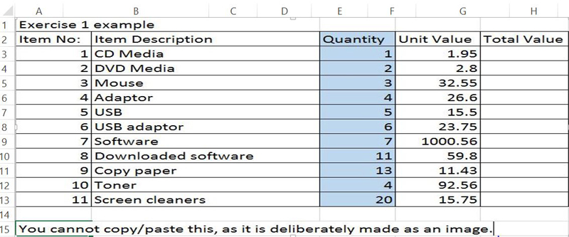
5	Enter the data from Exercise1 into the matching rows and columns. Use column widths to fit the data.
6	Create borders for the 10 items.
7	Fill colour the column you just added light blue.
8	Change the column widths to fit the headings.  Also the Wrap Text command
9	Decimal places - round up to two for places for all cells.
10	Using a formula in cell H3, fill in the answer. =sum(e3*g3)
10	Use the Fill series to complete the answers for the other items.
11	Finally add up the column. (=sum(h3:h11). In A14 type in Total.
12	Do a data sort, of the items in column B alphabetically.
13	Use a formula to multiply across and then do a fill down, then do a total.
14	Remove the unwanted columns C, D and E. See the line totals do not change. Instead the formula adjusts to the deleted columns.

Use this data source: